Compass/Wind

Compass/Wind #

Compass #

The compass is an optional module for the S2 interface, a magnetic sensor of the latest design, which allows an accuracy of up to one degree deviation with an optimal installation position and calibration. The magnetic sensor measures the earth’s magnetic field in 3D, i.e. in all 3 spatial directions, and has a tilt angle correction (tilt compensation). The sensor gets the inclination data from the AHRS module. For this it is necessary that the sensor calibration of the AHRS sensor is carried out once in its installation position, preferably in flight attitude. It is not necessary to activate the AHRS feature.

The magnetic sensor must be firmly connected to the aircraft in the correct position, the symbolism on the sensor shows an aircraft symbol with tail and wings, this must match the real aircraft and the lettering ‘Top’ must point upwards. There must not be any metal in the vicinity at the installation site, 20 better than 30 cm distance are minimum distances to deliver good results. The compass should not show more than 15°, better only 10° deviation (deviation) in any direction. A good position in a narrow glider fuselage, self-launchers or two seaters with lots of controls, cables and steel parts and various fittings is not easy to find. The cable should not be longer than two meters and should be point-to-point. If a flap sensor is also installed, pins 3 and 4 on interface S2 must only run to the magnetic sensor. Do not use an Y-Piece for an optional flap sensor but the S2-Extender if you got both. Otherwise, reading errors and even failure of the compass are possible.

For reasons of space, the display of the magnetic heading is currently only supported in the retro display or the UL style.
In the following menu items, its settings as well as the calibration of the sensor or the compensation of the deviation can be carried out.

Sensor Option #

[Disable]
[Enable I2C]
[Enable I2C no Tilt Comp.]
[Enable CAN Sensor]

With this, the type of magnetic sensor can be selected or the sensor can be switched off. By default, the magnetic sensor is switched off [Disable]. In the [Enable I2C] setting, a simple magnetic sensor connected to S2 with an I2C interface is selected, which compensates for the tilt angle (English Tilt Compensation). In the setting without tilt compensation in the next point, the usual compass rotation error up to an inversion of the display values can be expected. This setting is essentially only for test purposes, e.g. for a test setup on the top of a car. The [Enable CAN Sensor] setting enables the use of a new magnet sensor type with CAN interface as well with tilt compensation, which means that the serial interface on S2 remains free and can be used for other purposes, e.g. for the serial connection to an OpenVario. Furthermore, there is no restriction on the cable length for the CAN interface (max. 2 meters with I2C), the CAN magnetic sensor can therefore be installed at any point.

Note CAN: When selecting the CAN type, the CAN interface must be switched on in the system menu, the setting 1000 Kbit is recommended, other data rates are also possible. The sensor should also be plugged in when the compass is switched on, otherwise the software will query the module regularly, which will generate unnecessary CPU load in the event of an error.

Sensor Calibration #

[Cancel]
[Start]
[Show]
[Show Raw Data]

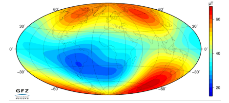
With this option, the measuring range of the magnetic sensor is calibrated in the same way as you know it from the compass module of a mobile phone. The calibration must be carried out again if the strength of the earth’s magnetic field changes, this is the case, for example, if you move to a different region on the globe. Normally, it is sufficient to carry out the calibration once.

For the purpose of calibration, the sensor must be swiveled in all spatial directions, which must be done before the sensor is permanently installed in its installation position at a location that is as free of metal or magnets as possible. The minima and maxima of the magnetic field strength in the individual spatial directions X,Y,Z are recorded and permanently stored in the non-volatile memory of the XCVario. Calibration is complete when the three displayed scale values (X, Y, Z scale) are close together and no longer change. In the sensor dialog, the measured field strength for the individual directions X,Y,Z is displayed live as a percentage of the maximum value of 2 gauss to the right of the scaling value in brackets.

example:

X Scale=95.2 (-5.2)
Y-Scale=100.4 (3.9)
Z-Scale=102.1 (13.9)

The best results are achieved if you calibrate the 3 directions individually and make sure that each direction X,Y,Z displays the maximum possible positive field strength once, e.g. (+18.5), and then and in the opposite direction, i.e. rotated 180 degrees, and with that the maximum negative display shows eg (-18.5). This is to be carried out for all 3 spatial directions in both directions. The corresponding spatial direction will turn green if the maximum values have been reached. This is the case when the other two directions are at zero or close to zero (display value less than 1.0), the other two direction sensors are then orthogonal to the earth’s magnetic field. A small graphic with maxima and minima, as well as the current measured values for the six directions X,Y,Z, positive and negative, makes calibration easier.

The X-axis of the sensor runs across the board (i.e. along the short side), the Y-axis along it (along the long side), and the Z-axis runs exactly perpendicular to the surface of the board.
Attention: The inclination, i.e. the inclination of the field line of the magnetic field to the earth’s surface, is between 62° and 70° in Germany (steeper in the north), the sensor for calibration is therefore at an angle of about 35°, namely inclined to the south, compared to the horizontal hold to capture the maximum value. Once you have found this, you rotate the sensor in exactly this position by 180° around its own axis, where this value is inverted. Then the sensor is rotated 90° in a different direction for the next axis.

The saved results of the calibration can be viewed at any time under the [Show] option.

With “Show Raw Data” the raw measured values, the sensor data, can be delivered in real time. An example is below:

X = 3397 
Y = 1874 
Z = 5420 
Raw magn H= 48.0 uT
Cal magn H= 48.5 uT

Here, the X, Y and Z values are the digital values of the AD converter for all three spatial directions. The value 8192 corresponds to 1 Gauss or 100 µT. And the “Raw Magn H” is the sum of squares of the values, i.e. the amount of the field strength in µT. The normal field strength in Germany is around 49 µT and should show around this value unaffected. The “Cal magn H” is shown when the sensor is fully calibrated, and should not deviate more than 2% from the raw value, if the difference is much more, this can indicate an incorrect calibration.

Note: No meaningful directions can be determined without the sensor calibration, so the display remains switched off until then. A faulty, incomplete calibration can lead to deviations in the magnetic heading.

Setup Declination #

0°

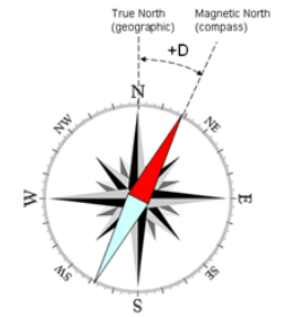
The local spatial variation or declination, source e.g. ICAO map or from airfield data on the Internet, can be taken into account with this parameter. A negative spatial declination, for example -2 degrees, corresponds to a deviation of the magnetic needle to the west. A positive spatial declination of e.g. 2 degrees corresponds to a deviation of the magnetic needle to the east. This setting can make sense if you start at a different location with a different local variation without wanting to carry out a new calibration.

Auto-Deviation #

[Disable]
[Enable]

When “Auto-Deviation” is switched on, the deviation is determined automatically, so it does not need to be compensated for manually, as is possible in the following point. This setting is part of the new method for wind calculation TAWC (Tesla Assisted Wind Calculation), which uses the direction information from the earth’s magnetic field, but calculates the compensation for the deviation in a control loop with the help of the wind information from the circling flight. The wind triangle is fed with the basic vector and the wind from the circling flight, and the result is a calculated vector for the heading and the airspeed, with which the deviations in the compass and the airspeed can be perfectly adjusted. The determined values are saved in the non-volatile flash memory approximately every hour. The procedure can only be used if there is at least a crank share of 20%. In pure straight flight, e.g. in a UL, manual deviation compensation at the compensation station is to be used.

Setup Deviations #

This compensates the deviation of the compass in its installation position in the aircraft. Each direction can be set separately via the dialog. This corresponds to the step-by-step creation of a deviation table; the software uses these values to carry out an approximation for all directions. To compensate for the deviation on the ground, the aircraft must be rotated precisely in eight different directions with the wings level. For this purpose, some airfields have a compensation area with a compass rose attached to the ground, which makes this easy to do. If this is not an option, the direction can be determined with the help of an accurate compass, e.g. on the wing.
For complete compensation, all 8 directions must be selected and the calibration started and ended by pressing a button. After confirmation, the value is stored in non-volatile memory and you can move to the next direction.

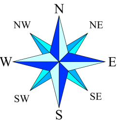
Direction: 000
Direction: 045
Direction: 090
Direction: 135
Direction: 180
Direction: 225
Direction: 270
Direction: 315

Two different effects are compensated for in the specific installation position, the so-called “soft iron effect” which is caused by the influence of non-magnetic metals on the earth’s magnetic field, such as nickel or iron, and bends the magnetic field. There are also the “hard iron effects”, metals which are magnetic themselves, i.e. produce their own magnetic fields and normally emanate from magnets such as a loudspeaker.

Show Deviations #

The deviation values can be displayed under this point, for all eight directions for which the deviation was saved, whether it was determined manually through compensation as in the previous point, or calculated using the AutoDeviation feature. A small graphic illustrates the course of the deviation curve. Ideally, the curve should be continuous and have a sine period without further oscillations.

Reset Deviations #

[Cancel]
[Reset]

An existing deviation table as created in the previous point can be deleted here.

Setup NMEA #

Setting the NMEA sentences generated by the compass module.

Magnetic Heading #

[Disable]
[Enable]

Turn on the generation of NMEA sentences for the magnetic course, which points in the direction of magnetic north. The corresponding NMEA sentence for this is $HCHDM.

True Heading #

[Disable]
[Enable]

To generate the NMEA for True Heading, according to $HCHDT, a spatial variation (declination) must be recorded and the calibration carried out.

Damping #

3.00 sec

Damping calms down the compass display, the default is 3 seconds, which is usually sufficient to get a stable display. If the displayed value is not stable in individual cases, e.g. due to electrical lines or other sources of interference, the damping can be increased slightly. The settling times increase accordingly.

I2C Clock #

100 KHz

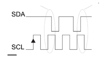
The clock of the I2C bus (SCL) to the magnetic sensor, which is outside the housing, can be set here. 100 KHz is the manufacturer’s recommendation for the chip. If, for example, problems arise with this due to long lines, such as a sensor not being found during calibration or no display being visible, the frequency can also be lowered.

Show Settings #

Shows an overview of the most important settings and whether the measuring range has been exceeded (sensor overflow).

Wind Calculation #

[Disable]
[Straight]
[Circling]
[Both]

With this option the wind calculation is switched on. The information is shown in the retro display (below the airspeed).
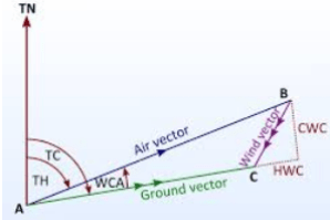
For wind in straight flight (Straight setting), the compass must be installed and functional, and the sensor calibration must be performed. The wind is calculated as vector subtraction of the air vector from the true heading (TH) of the compass and the airspeed, as well as from the GPS signal of a connected FLARM the ground vector from ground speed and the true course (TC), the course over ground. The deviation can be compensated on the ground or automatically determined in flight. The XCVario must also be connected to a Flarm. The wind in level flight is an important piece of information, since with crank percentages of perhaps only 20%, a glider will be in level flight most of the time. A good accuracy of the compass is important here, the high-resolution 3D magnetic sensor, available as an additional module for the XCVario hardware since series 21 that supports this.

Below is a comparison of the wind display of both methods over an entire flight day on February 7th, 2022 (https://www.weglide.org/flight/178203), at the altitude of the flight with the east wind with approx. 20 km/h in the west from 120° and turning east to south by 150° were announced. Both methods meanwhile give values with good agreement:

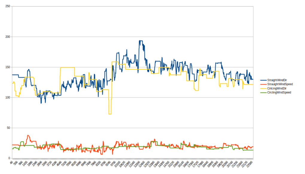
Note: The straight flight setting for the wind calculation has been test in flight and has been optimized with the help of simulations, so it is still under minor development. The releases since summer 2023 look promising. Once the sensor is well calibrated and far enough from metal all is fine.
The wind calculation in circling, is fully stable. The method is identical to the method implemented in XCSoar or Cumulus, from which it originally came.
In the ‘Both’ setting, the wind that has just been calculated is always displayed. Depending on the flight status, circles or straight ahead, the corresponding calculations are carried out here.

Display #

[Disable]
[Wind Digits]
[Wind Arrow]
[Wind Both]
[Compass]

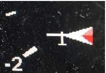
Under the “Display” setting, either the current wind can be displayed digitally [wind digits], e.g. 90°/25 in the format of wind direction/wind force in the retro-style display (below IAS/TAS), or as a small wind arrow within the display [Wind Arrow], or both ways [Wind Both]. By default, the wind indicator is disabled [Disable].

In addition, in the [Compass] setting, the compass course can also be selected and displayed. If there is no wind calculation, e.g. on the ground or during the first calculations, the compass course is always displayed instead of the digital wind. The wind is always displayed in the unit selected for the airspeed.

Arrow Ref #

[North]
[Mag Heanding]
[GPS Course]

The “Arrow Ref(erence)” determines whether the wind arrow (Engl. Arrow), relative to the north direction, to the compass course or direction of the longitudinal axis of the aircraft [Mag. Heading] (only possible if a magnetic sensor is present), i.e. to the longitudinal axis of the aircraft, or relative to the GPS course [GPS Course] over the ground. The wind arrow is only displayed in retro-style display mode. For relative plots, a small airplane symbol is drawn at the wind’s tip.

Straight Wind #

Filters #

Airspeed Lowpass #

0.020

The airspeed sensor is continuously calibrated during wind measurement. The low-pass factor determines the speed at which the calibration is adjusted. The default value of 0.020 or 2% means a calibration change of 2% per second. Normally, the default value does not need to be adjusted.

Deviation Lowpass #

0.020%

The deviation of the magnetic sensor is also continuously calibrated during wind measurement. The low-pass factor determines the speed at which the calibration is adjusted. The default value of 0.020 or 2% means a calibration change of 2% per second. Normally, the default value does not need to be adjusted.

GPS Lowpass #

1.0 sec

This value is used to subsequently filter the course information from the GPS in order to obtain an identical time behavior with the compass. The default value is still being optimized at the moment and may change slightly.

Averager #

60

This determines the number of measurements that are relevant for the averaging of the measurements. Measurements are taken every second, a value of 20 (default) means an average over the last 20 seconds. A smaller setting makes the wind calculation more nervous, deviations in the course, e.g. due to side slip, are immediately apparent. At a higher setting, temporary deviations are averaged out.

Limits #

Deviation Limit #

30 °

The correct deviation of the magnetic sensor is an important parameter and can be calculated automatically with “AutoDeviation” using the circling wind. The tolerance indicates how far the calculated deviation for the current direction may deviate from the last saved value. In the case of values above this, the current wind measurement is rejected as implausible. The default is 30%. Normally, the value does not need to be adjusted.

#

Sideslip Limit #

2.0°

The wind calculation requires a precise heading, which is only guaranteed if the thread remains exactly in the middle. Even with deviations of a few degrees, the accuracy of the wind calculation decreases. Typically, gliders oscillate a few degrees around the vertical axis with each correction due to the roll turning moment, which varies in strength depending on the model. So that the sideslip has little or no influence on the wind calculation, the XCVario continuously calculates the sideslip angle from the sensors and only uses those wind measurements that were obtained at a sideslip angle within a tolerance that can be configured here. The smaller this value, the more precise the wind calculation, but the fewer measurements will fall within the tolerance band. For checking, the slip angle can be shown live in the field of the speed display (IAS/TAS) in the retro display. By default, a maximum sideslip angle of 2 degrees (to the left and to the right) is configured. Values ​​down to 1 degree have already been successfully tested.

Course Limit #

7.5°

The course limit specifies the maximum deviation in degrees per second for level flight up to which the wind calculation is carried out. A measurement at higher turning speeds than the configured value is rejected as containing errors. The default is 7.5 degrees per second.

AS Delta Limit #

15 km/h

The AS Delta Limit specifies the maximum deviation in km/h for the flight speed in level flight, up to which the wind calculation is carried out. A measurement with a higher variance of the speed than the configured value is rejected as containing errors. The default is 15 km/h change per second.

Straight Wind Status #

The status screen shows information on the straight flight wind calculation, such as the input parameters, e.g. the GPS status, deviations in ground speed and airspeed within the measurement window, the underlying compass deviation and more can also be used for diagnosis if the measurement does not work.

Straight Wind enabled : Yes [ No ] (Feature active or not)

Status : Initial [ Calculating ] (status of calculation)

GPS Status: Good [Bad ]

AS C/F: +1.000%/1.000% (Airspeed calibration Info)

Last Wind : 93°/25 (Direction and wind strength in the set unit for speed)

MH/Dev: 68.00/+7.23: (Magnetic Heading and corresponding Deviation)

Wind Age : 120 sec (Age of the last wind measurement)

Circling Wind #

When circling the wind calculation, only a few can be adjusted, the procedure is quite simple. The calculation is based purely on the GPS data, a compass module is not necessary for this, therefore also possible on devices of the 2020 series, without a second S2 interface. A Flarm as a GPS data source is the prerequisite for this. During the calculation, the vectors of the ground speed are evaluated and the wind vector is calculated from the directions of the maximum and minimum ground speed. The method also works for circles that are not quite circular; a relatively constant speed when circling is advantageous. The measurement is improved by intelligent filtering (simplified Kalman filter) over several circles, using the quality factor of the measurement from the correlation of the direction of the minima and maxima of the measured speed values. Normally, two to three circles are enough for a precise value, and after just one circle, the wind is initially displayed.

Circling Wind Status #

The status screen shows information about the circling wind calculation. This display element can be left again by pressing a button. The information is updated by turning the knob.

Circling Wind enabled : Yes [ No ] (Feature enabled or not)

GPS Status : Good [ Bad ] ( The GPS status)

GPS Satellites: 8 (number of satellites )

Number of Circles: 2.52 (Number of circles that have been rotated since the start of the measurement )

Last Wind : 93°/25 (Current direction/wind strength in the set unit for speed)

Wind Age : 20 sec (age of last wind measurement)

Quality : 95% (Factor for the quality of the measurement (0..100%)

Status: sampling (status of wind calculation)

Flight Mode: circling L (Flight mode, calculations are only made when circling)

Max Angle Delta #

90°

The maximum permissible angle difference of the normalized directions for the maximum and minimum speed over ground (ground vector) can be set here. The default is 90 degrees, beyond which a wind calculation no longer makes sense, so a circle with an angle difference of more than 90 degrees is discarded for the wind calculation.

Averager #

5

This determines the number of measurements that are relevant for averaging the wind measurements when circling. The measurement is made after each complete circle. A value of 5 (default) means an averaging over the last 5 circles. A smaller setting makes the wind calculation more nervous, a higher setting dampens temporary outliers, e.g. due to speed fluctuations while circling.

Wind Logging #

[Disable]
[Enable WIND]
[Enable GYRO/MAG]
[Enable Both]

With this setting, the wind logger can be activated, which is used to develop and optimize the feature, and generates NMEA-like data sets with the $WIND identifier in the normal NMEA data stream of the XCVario. The data record contains a time stamp (second), the basic vector (°, km/h), the airspeed vector, the current wind calculation and the average wind, the last circle wind calculation, the airspeed correction, the flight mode, the GPS status and the deviation.
In order to be able to evaluate the data after the flight, the “NMEA logger” must be set to “On” in addition to this setting to Enable in the XCSoar settings under System→Settings→Logger.
An .nmea file is then stored in the XCSoarData, the logs directory, which contains all the information that the XCVario has sent to XCSoar, including the $WIND data record.

The GYRO/MAG setting outputs additional data fields with the X,Y,Z raw values of the acceleration, the gyrometer and the magnetic sensor.

Beispiel:

$WIND;9747;214.8;115.9;153.1;136.3;58.9;116.6;58.9;116.6;89.8;26.2;5.0,1,1,-16.8